Last year, we have published a paper on feature extraction with Gaussian Mixture Model (see pdf). This work has been continued these past months by Adrien Lagrange during its internship at the lab, under co-supervision of Manuel Grizonnet (CNES).
We have extended the linear algebra to save computational resources during the main step of the optimization. A paper has been submitted and details of the computation can be seen on HAL. As usual, the python code is freely available from the github of Adrien.
Furthermore, the algorithm have been implemented in an Orfeo Toolbox module. It is now available from the external modules webpage.
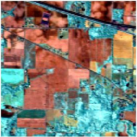
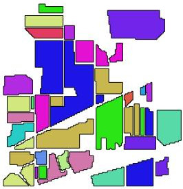
In this post, I am going to illustrate how it works and behaves on the famous AVIRIS data set. See images falseColor and ref. The image has 220 spectral bands and a size of 145 \(\times\) 145 pixels. The original data can be download:


How it works ?
otbcli_TrainGMMSelectionApp -helpSo we need an image, a reference file and to choose what is the method we are going to use. I refer to the aforementioned paper for details ;)
Here, we are going to apply the feature selection algorithm with the following parameters:
- Criteria: the Kappa coefficient and the Jeffreys-Matusita distance.
- Method: forward.
- Number of variables: 30
- Number of samples per class: 50
Let’s go:
for crit in jm kappa
do
otbcli_TrainGMMSelectionApp -io.il ./images/aviris.tif \
                -io.vd ./images/ref.shp \
                -io.confmatout ./images/res_simu_npfs/confu_${crit}.txt \
                -io.out ./images/res_simu_npfs/model_${crit}.txt \
                            -sample.mt 50 \
                -sample.bm 0 \
                -gmm.method forward \
                -gmm.crit ${crit} \
                -gmm.varnb 30 \
                -rand 0
done
Then we can extract the number of selected features, and the global accuracy, for each criteria, from the txt files:
import linecache
import scipy as sp

for name_ in ["kappa","jm"]:
    # Selected bands
    filename = "images/res_simu_npfs/model_{}_selection.txt".format(name_)
    NumberOfSelectedBands = int(linecache.getline(filename,2).split()[1])
    SelectedBands = linecache.getline(filename,2+NumberOfSelectedBands).split()
    print("Number of selected band for {} criteria: {}".format(name_,NumberOfSelectedBands))
    print("Selected Bands:")
    print(SelectedBands)
    print("")
Number of selected band for kappa criteria: 8
Selected Bands:
['27', '35', '74', '133', '40', '203', '10']
Number of selected band for jm criteria: 30
Selected Bands:
['180', '131', '71', '12', '38', '34', '167', '61', '119', '47', '89', '198', '26', '6', '4', '139', '116', '144', '96', '32', '163', '197', '146', '46', '28', '130', '135', '30', '59']
import linecache
import scipy as sp
import matplotlib.pyplot as plt

for name_ in ["kappa","jm"]:
    # Confusion Matrix
    filename = "images/res_simu_npfs/confu_{}.txt".format(name_)
    confusionMatrix = sp.genfromtxt(filename,delimiter=',',skip_header=2)
    OA = sp.diag(confusionMatrix).sum()/confusionMatrix.sum()
    print("Overall Accuracy for criteria {}: {}".format(name_,OA))
Overall Accuracy for criteria kappa: 0.81195335277
Overall Accuracy for criteria jm: 0.607871720117
From the classification accuracy, we can see that the JM criteria performs worse than the Kappa criteria (similar conclusion would have been done if F1 mean or OA criterion have been used). JM is widely used in remote sensing, but it might perform badly in some cases where the Gaussianity is not fulfilled, as illustrated in these short example.
It is also possible to get the learning curves, i.e., the Kappa/JM value in function of the number of selected bands.
import linecache
import scipy as sp
import matplotlib.pyplot as plt
import matplotlib
matplotlib.style.use('ggplot')

for name_ in ["kappa","jm"]:
    # Selected bands
    filename = "images/res_simu_npfs/model_{}_selection.txt".format(name_)
    crit = []
    for lineNumber in range(35,65):
        crit.append(linecache.getline(filename,lineNumber).split()[1])
    plt.figure()
    plt.title("Learning curves for {}".format(name_))
    plt.plot(range(1,31),crit,'o')
    plt.grid(b=True)
    plt.savefig("images/learning_curve_{}.png".format(name_))
    print("[[./images/learning_curve_{}.png]]".format(name_))


A global maximum is reached with the Kappa for 8 extracted features. If we look to the table tab, this is the highest number of features for which the number of training samples is higher than the number of parameters to estimate.
For the JM criteria, the value still increased (slowly) for 30 features. /Note: rather than selecting the maximum value of the criteria, we could stop when the increased of the criteria is too small. It can be done in two steps with the module./
| # of variables | # of parameters to estimate |
|---|---|
| 1 | 2 |
| 2 | 5 |
| 3 | 9 |
| 4 | 14 |
| 5 | 20 |
| 6 | 27 |
| 7 | 35 |
| 8 | 44 |
| 9 | 54 |
| 10 | 65 |
Classify the whole data set
Now it is possible to classify the whole image:
otbcli_PredictGMMApp -helpBy default, the number of selected for the prediction corresponds to the number of variables for which the criteria is maximum. But it is possible to change it with the option -varnb. To classify the image using the model obtain with Kappa
otbcli_PredictGMMApp -in images/aviris.tif \
             -model images/res_simu_npfs/model_kappa.txt \
             -modeltype selection \
             -out images/res_simu_npfs/thematic_aviris.tif
The resulting images is given in fig:thematic. Off course, spatial information should be included in the classification process. But the subject of this post is about feature extraction: with only 8 features from 220, and 50 training samples per class we get an OA of 81 % … so that’s all folk !

And with SVM ?
If we do the classification with the classifier SVM ? Using the default implementation of OTB (LIBSVM), it can be done with the following command:
otbcli_ComputeImagesStatistics -il ./images/aviris.tif -out stat.xml
otbcli_TrainImagesClassifier -io.il ./images/aviris.tif \
                 -io.vd ./images/ref.shp -io.out .images/res_simu_npfs/model_svm.txt \
                 -io.imstat stat.xml \
                 -classifier libsvm \
                 -classifier.libsvm.k rbf -classifier.libsvm.opt 1 \
                 -rand 0 -sample.mt 50 -sample.bm 0 \
                 -io.confmatout .images/res_simu_npfs/confu_svm.txt
Then the OA is again found by
import scipy as sp
filename = "images/res_simu_npfs/confu_svm.txt"
confusionMatrix = sp.genfromtxt(filename,delimiter=',',skip_header=2)
OA = sp.diag(confusionMatrix).sum()/confusionMatrix.sum()
print("Overall Accuracy for SVM: {}".format(OA))
Overall Accuracy for SVM: 0.711370262391
What ? We are better than the super SVM ! Ok, it’s my website … But if you check the JSTARS paper, when the number of samples is very low, we are usually better. But when the number of training samples becomes large, then SVM (and RF) tends to be better in terms of classification accuracy.
Comments
comments powered by Disqus